Go beyond predictive modeling : Accurately compute interventions and counterfactuals with Double Machine Learning


TL;DR
- Double Machine Learning can be used to learn unbiased estimates of causal effects
- decisionOS by causaLens offers the only package that allows learning unbiased structural causal models using Double Machine Learning, providing accurate answers to interventional (‘what-ifs’) and counterfactual (‘what-would-have’) questions
- causaLens has spent many hours of R&D time implementing a model-agnostic Full Graph Double Machine Learning training framework to train Structural Causal Models
- This blog will outline how Double Machine Learning can be applied to an example use case in the medical industry and how it significantly outperforms traditional machine learning methods such as XGBoost
Why Double Machine Learning?
Accurate predictions are a key part of creating effective data science solutions. However, data science work delivers the most value when it goes beyond predictions offering explainable, actionable insights to business stakeholders. To do this, solutions need to be able to understand causal effects, so that interventional (‘what-if’) and counterfactual questions can be asked of the model and unbiased results returned. Without this ability to query the model, data science solutions often remain in the lab and are not used for decision making in the real world.
To create an accurate model which allows these questions to be asked, a Structural Causal Model (SCM) should be used. SCMs are able to capture causal relationships between all of the features within a given dataset, including the target. However, simply using an SCM is not sufficient, a method for training SCMs without introducing bias is also required.
Empirical risk minimization is the standard approach to training predictive models and often causal models. Unfortunately, models trained in this way struggle to distinguish between causal and non-causal relationships (e.g. spurious correlations). This means models perform poorly in the presence of confounding variables and are also prone to overfitting, leading to solutions which generalize poorly.
In contrast, Double Machine Learning (DoubleML), also referred to as debiased machine learning, offers a method of training causal models which is able to create unbiased estimates of causal effects, and is far less prone to overfitting. This can come at the expense of some pure predictive power, but the ability to accurately compute counterfactuals is a significant gain.
decisionOS by causaLens offers the only package for training SCMs using DoubleML. causaLens has spent many hours of R&D time implementing a model-agnostic Full Graph DoubleML training framework to train the SCMs. This approach has shown significant value across a number of use cases in a range of industries.
This blog will outline how Double Machine Learning can be applied to an example use case in the medical industry and how it significantly outperforms traditional machine learning methods such as XGBoost.
Use case example
A medical institute is trying to quantify the effects that a medication has on a patient’s life expectancy after they have been diagnosed with a given disease. Data has been collected from an observational study. In the study, patients were given a specified dose of medicine and the period between the administration of the medicine and their death was recorded. The age of the patients at the point of diagnosis was also recorded. Since this was not a Randomized Control Trial (RCT), it is clear that the age of patients likely had an effect on the amount of medicine prescribed, as well as their life expectancy. The causal graph for this data is shown below.
Immediately, it is clear to see that age confounds both medicine dosage and life expectancy; the disease does not feature in the causal graph as, in this instance, there was no control group within the dataset, everyone had been diagnosed with the disease.
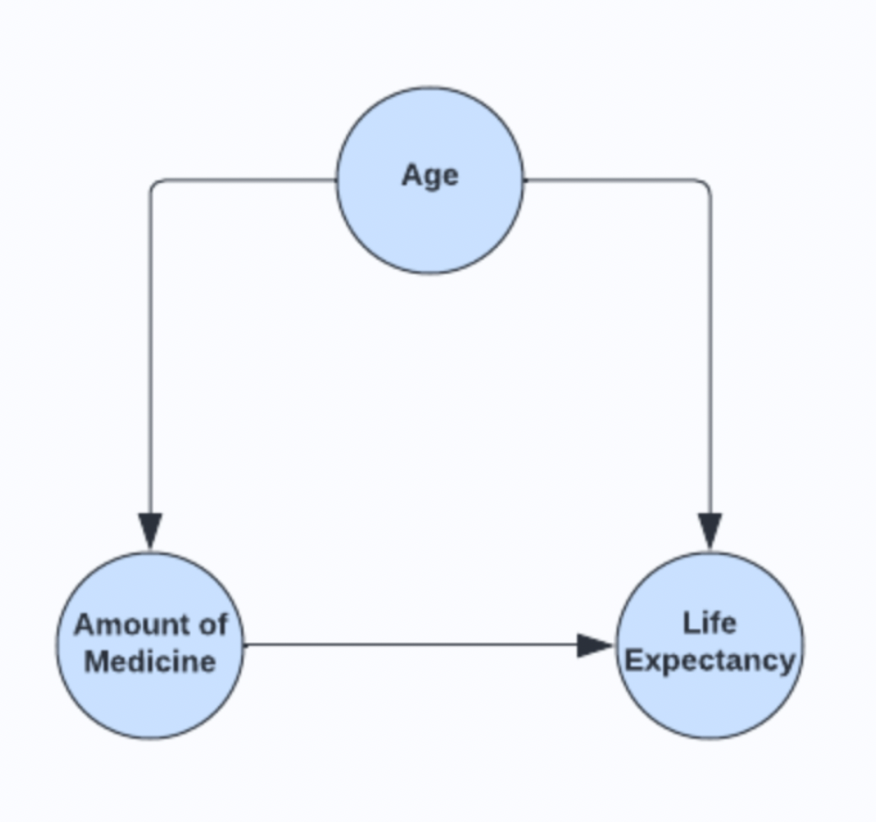
Figure 1: Age is a confounding variable for the relationship between Amount of Medicine and Life Expectancy
For a given participant P, the data tells us they received 82mL of medicine at 18.2 years old and lived for 34.8 years. From this information, we may want to understand e.g. how long would individual P have lived, if they received 500mL medicine?
Figure 2 shows the trends across the data and how the individual of interest is out of sample.
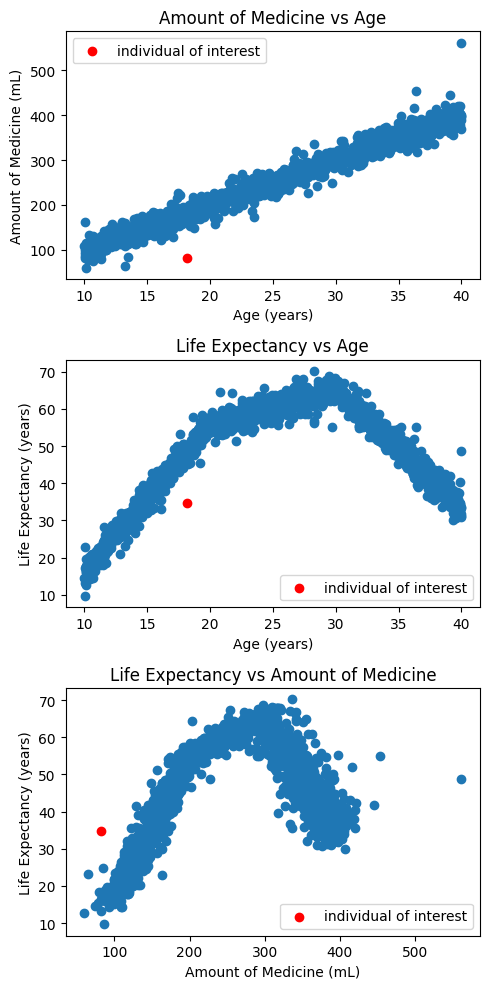
Figure 2: Distribution of variables within the dataset
The challenge with classical ML estimators
A naive approach to answering this question is to use a classical ML estimator, such as XGBoost, to regress life expectancy on age, at diagnosis, and the amount of medicine administered. To assess estimator performance, data can be divided into training and testing samples. The XGBoost model produces 1.2 mean absolute error (MAE) on the test set, so it appears to model the data accurately.
To perform the counterfactual query, the exogenous noise for the life expectancy needs to be computed for individual P. This estimator can then be used to predict life expectancy for the values of interest [18.2 years age at diagnosis, 500mL dose]. Finally, the results are added with the abducted exogenous noise. As this is a synthetic example, the result can be compared to the ground truth, producing a 41.8 MAE – significantly larger than MAE observed on the test set. So, what causes the large discrepancy?
The answer is that the approach is fundamentally flawed. While the trained estimator may produce accurate predictions on the testing set, it produces biased predictions for interventional (or counterfactual) queries. The reason for this lies in the different underlying data distribution in the training and testing samples, and the interventional samples. More simply, the classical ML estimator is only able to represent the observational distribution p(Y|T, X). But once the treatment is intervened on, the observational distribution is no longer sufficient and an estimate of the interventional distribution p(Y|do(T), X) is required. The following section outlines this in more detail.
Why is it difficult to learn the interventional distribution?
The causal graph below describes the data generation process for the training data. There is a single causal path between T (medicine dose) and Y (life expectancy), but these variables are also related through the backdoor path T<-X->Y. An estimator trained using a classical approach (i.e. empirical risk minimization), is unable to disentangle which information comes solely from T when learning the function for T -> Y as the influence of X (age) on T is not properly accounted for. It will have learnt a relationship which is a combination of the true causal effect of T on Y, and its association with Y through X.
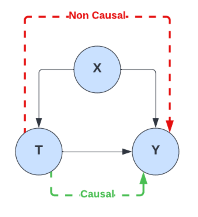
Figure 3: Causal and backdoor paths within the causal graph
Now, consider the data generation model for the counterfactual question. An intervention on node T is required to compute the value of Y for a specific value of T. This means that the causal link between X and T is severed and the backdoor path T<-X->Y is removed. The correlation between T and Y, present in the observational dataset that the classical ML estimator learns during training, no longer holds, leading to biased and inaccurate results.
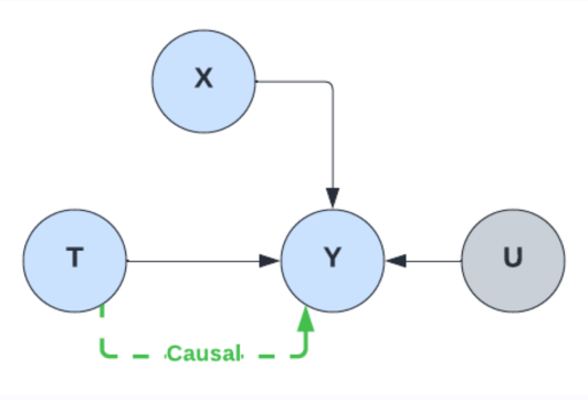
Figure 4: Intervening removes the backdoor parth within the causal graph (U is the exogenous noise on Y)
Classical estimators often rely on a fundamental assumption of independent and identically distributed data (i.i.d). This ubiquitous assumption plays a critical role when attempting to use estimators for interventional analysis as the intervention changes the data distribution. Mathematically, this can be described using do-calculus, namely: P(Y|T) does not equal P(Y|do(T)).
In practice, it means that the XGBoost model will perform well, as long as the distribution of test data is identical to the distribution of the training data. As the correlation between T and Y in the testing data is the same as it is in the training data, the XGBoost model did perform well. However, since the correlation changes when performing a counterfactual query (the backdoor association T<-X->Y is removed), the results will be incorrect. This could lead to potentially life threatening consequences in this instance. At the very least, suboptimal decisions can be expected.
So, how can this challenge be overcome?
Using doubleML to produce unbiased interventional and counterfactual predictions
Double Machine Learning (DoubleML) provides a framework to estimate unbiased relationships between variables. It works by enabling the model to disentangle causal and non-causal dependencies, ensuring only causal relationships are learnt.
To illustrate advantages of training an SCM with DoubleML, causaLens proprietary framework CausalNet is used to create and train an SCM using the same data. The test set MAE is 5.78, significantly larger than the XGBoost performance. The result of the counterfactual query (do(T=500mL), given [X = 18.2 years, T = 82mL, Y = 34.8 years]) is 76.2 years, with the MAE compared to ground truth of only 0.35 years vs 41.8 for XGBoost. Hence, CausalNet was slightly worse than XGBoost on the test set in a purely predictive task, but it completely outperforms XGBoost on the counterfactual.
XGBoost learns the observational data distribution well but completely fails to learn the interventional distribution. The counterfactual, which is derived from the interventional distribution, is the important quantity when trying to improve decision making and so trading off some pure predictive power to improve this is worthwhile. Learning an SCM that captures both distributions is more powerful for real world use cases.
Overall, it is the combination of an SCM and a debiased training method that allows this improved performance when computing counterfactuals.
While the DoubleML framework has been available for a number of years and is offered through open-source packages, such as EconML and DoubleML, so far it has been mainly used for unbiased treatment effect estimation. Extending this so that full Structural Causal Models with arbitrary Directed Acyclic Graphs (DAGs) can be learnt is significantly more complex. causaLens has spent a significant amount of time implementing a model-agnostic Full Graph DoubleML training framework to train the SCMs. decisionOS is the only place where this implementation is available.
Once an unbiased SCM has been learnt, it can be used by causaLens proprietary Decision Intelligence Engines (DIEs). For example, it may be used to identify an optimal action, using Algorithmic Recourse, or to identify a true root cause using the Root Cause Analysis engine. It can also be used to perform accurate what-if analysis, or estimate the impact of previous actions.
Conclusion
Creating models which are able to reason about the world requires a cause and effect understanding of data. To do this, models need to be able to provide unbiased estimates which can be actioned. Training an SCM using DoubleML is the only way to ensure the model remains accurate, even when the interventional distribution does not equal the observational one. decisionOS by causaLens makes it very easy to create and train unbiased SCMs, significantly enhancing decision-making capabilities across the enterprise.
If you’d like to learn more, you can view our Demo Hub or request a Free Trial of the leading Causal AI platform.